Normal distribution

Normal distribution

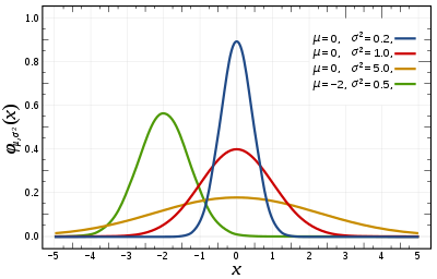
Probability density function The red curve is the standard normal distribution.
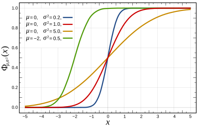
Cumulative distribution function
Notation	${\displaystyle {\mathcal {N}}(\mu ,\sigma ^{2})}$
Parameters	${\displaystyle \mu \in \mathbb {R} }$ = mean (location) ${\displaystyle \sigma ^{2}\in \mathbb {R} _{>0}}$ = variance (squared scale)
Support	${\displaystyle x\in \mathbb {R} }$
PDF	${\displaystyle {\frac {1}{\sqrt {2\pi \sigma ^{2}}}}e^{-{\frac {(x-\mu )^{2}}{2\sigma ^{2}}}}}$
CDF	${\displaystyle \Phi \left({\frac {x-\mu }{\sigma }}\right)={\frac {1}{2}}\left[1+\operatorname {erf} \left({\frac {x-\mu }{\sigma {\sqrt {2}}}}\right)\right]}$
Quantile	${\displaystyle \mu +\sigma {\sqrt {2}}\operatorname {erf} ^{-1}(2p-1)}$
Mean	${\displaystyle \mu }$
Median	${\displaystyle \mu }$
Mode	${\displaystyle \mu }$
Variance	${\displaystyle \sigma ^{2}}$
MAD	${\displaystyle \sigma {\sqrt {2/\pi }}}$
Skewness	${\displaystyle 0}$
Excess kurtosis	${\displaystyle 0}$
Entropy	${\displaystyle {\frac {1}{2}}\log(2\pi e\sigma ^{2})}$
MGF	${\displaystyle \exp(\mu t+\sigma ^{2}t^{2}/2)}$
CF	${\displaystyle \exp(i\mu t-\sigma ^{2}t^{2}/2)}$
Fisher information	${\displaystyle {\mathcal {I}}(\mu ,\sigma )={\begin{pmatrix}1/\sigma ^{2}&0\\0&2/\sigma ^{2}\end{pmatrix}}}$ ${\displaystyle {\mathcal {I}}(\mu ,\sigma ^{2})={\begin{pmatrix}1/\sigma ^{2}&0\\0&1/(2\sigma ^{4})\end{pmatrix}}}$
Kullback–Leibler divergence	${\displaystyle {1 \over 2}\left\{\left({\frac {\sigma _{0}}{\sigma _{1}}}\right)^{2}+{\frac {(\mu _{1}-\mu _{0})^{2}}{\sigma _{1}^{2}}}-1+\ln {\sigma _{1}^{2} \over \sigma _{0}^{2}}\right\}}$
Expected shortfall	${\displaystyle \mu -\sigma {\frac {{\frac {1}{\sqrt {2\pi }}}e^{\frac {-\left(q_{p}\left({\frac {X-\mu }{\sigma }}\right)\right)^{2}}{2}}}{1-p}}}$[1]

Part of a series on statistics
Probability theory
Probability Axioms Determinism System Indeterminism Randomness
Probability space Sample space Event Collectively exhaustive events Elementary event Mutual exclusivity Outcome Singleton Experiment Bernoulli trial Probability distribution Bernoulli distribution Binomial distribution Exponential distribution Normal distribution Pareto distribution Poisson distribution Probability measure Random variable Bernoulli process Continuous or discrete Expected value Variance Markov chain Observed value Random walk Stochastic process
Complementary event Joint probability Marginal probability Conditional probability
Independence Conditional independence Law of total probability Law of large numbers Bayes' theorem Boole's inequality
Venn diagram Tree diagram
v t e

In probability theory and statistics, a normal distribution or Gaussian distribution is a type of continuous probability distribution for a real-valued random variable. The general form of its probability density function is $${\displaystyle f(x)={\frac {1}{\sqrt {2\pi \sigma ^{2}}}}e^{-{\frac {(x-\mu )^{2}}{2\sigma ^{2}}}}\,.}$$ The parameter ${\textstyle \mu }$ is the mean or expectation of the distribution (and also its median and mode), while the parameter ${\textstyle \sigma ^{2}}$ is the variance. The standard deviation of the distribution is ${\textstyle \sigma }$ (sigma). A random variable with a Gaussian distribution is said to be normally distributed, and is called a normal deviate.

Normal distributions are important in statistics and are often used in the natural and social sciences to represent real-valued random variables whose distributions are not known.^[2][3] Their importance is partly due to the central limit theorem. It states that, under some conditions, the average of many samples (observations) of a random variable with finite mean and variance is itself a random variable—whose distribution converges to a normal distribution as the number of samples increases. Therefore, physical quantities that are expected to be the sum of many independent processes, such as measurement errors, often have distributions that are nearly normal.^[4]

Moreover, Gaussian distributions have some unique properties that are valuable in analytic studies. For instance, any linear combination of a fixed collection of independent normal deviates is a normal deviate. Many results and methods, such as propagation of uncertainty and least squares^[5] parameter fitting, can be derived analytically in explicit form when the relevant variables are normally distributed.

A normal distribution is sometimes informally called a bell curve.^[6] However, many other distributions are bell-shaped (such as the Cauchy, Student's t, and logistic distributions). (For other names, see Naming.)

The univariate probability distribution is generalized for vectors in the multivariate normal distribution and for matrices in the matrix normal distribution.

The simplest case of a normal distribution is known as the standard normal distribution or unit normal distribution. This is a special case when ${\textstyle \mu =0}$ and ${\textstyle \sigma ^{2}=1}$, and it is described by this probability density function (or density): $${\displaystyle \varphi (z)={\frac {e^{\frac {-z^{2}}{2}}}{\sqrt {2\pi }}}\,.}$$ The variable ${\textstyle z}$ has a mean of 0 and a variance and standard deviation of 1. The density ${\textstyle \varphi (z)}$ has its peak ${\textstyle {\frac {1}{\sqrt {2\pi }}}}$ at ${\textstyle z=0}$ and inflection points at ${\textstyle z=+1}$ and ${\textstyle z=-1}$.

Although the density above is most commonly known as the standard normal, a few authors have used that term to describe other versions of the normal distribution. Carl Friedrich Gauss, for example, once defined the standard normal as $${\displaystyle \varphi (z)={\frac {e^{-z^{2}}}{\sqrt {\pi }}},}$$ which has a variance of ⁠${\displaystyle {\frac {1}{2}}}$⁠, and Stephen Stigler^[7] once defined the standard normal as $${\displaystyle \varphi (z)=e^{-\pi z^{2}},}$$ which has a simple functional form and a variance of ${\textstyle \sigma ^{2}={\frac {1}{2\pi }}.}$

Every normal distribution is a version of the standard normal distribution, whose domain has been stretched by a factor ${\textstyle \sigma }$ (the standard deviation) and then translated by ${\textstyle \mu }$ (the mean value):

$${\displaystyle f(x\mid \mu ,\sigma ^{2})={\frac {1}{\sigma }}\varphi \left({\frac {x-\mu }{\sigma }}\right)\,.}$$

The probability density must be scaled by ${\textstyle 1/\sigma }$ so that the integral is still 1.

If ${\textstyle Z}$ is a standard normal deviate, then ${\textstyle X=\sigma Z+\mu }$ will have a normal distribution with expected value ${\textstyle \mu }$ and standard deviation ${\textstyle \sigma }$. This is equivalent to saying that the standard normal distribution ${\textstyle Z}$ can be scaled/stretched by a factor of ${\textstyle \sigma }$ and shifted by ${\textstyle \mu }$ to yield a different normal distribution, called ${\textstyle X}$. Conversely, if ${\textstyle X}$ is a normal deviate with parameters ${\textstyle \mu }$ and ${\textstyle \sigma ^{2}}$, then this ${\textstyle X}$ distribution can be re-scaled and shifted via the formula ${\textstyle Z=(X-\mu )/\sigma }$ to convert it to the standard normal distribution. This variate is also called the standardized form of ${\textstyle X}$.

The probability density of the standard Gaussian distribution (standard normal distribution, with zero mean and unit variance) is often denoted with the Greek letter ${\textstyle \phi }$ (phi).^[8] The alternative form of the Greek letter phi, ${\textstyle \varphi }$, is also used quite often.

The normal distribution is often referred to as ${\textstyle N(\mu ,\sigma ^{2})}$ or ${\textstyle {\mathcal {N}}(\mu ,\sigma ^{2})}$.^[9] Thus when a random variable ${\textstyle X}$ is normally distributed with mean ${\textstyle \mu }$ and standard deviation ${\textstyle \sigma }$, one may write

$${\displaystyle X\sim {\mathcal {N}}(\mu ,\sigma ^{2}).}$$

Some authors advocate using the precision ${\textstyle \tau }$ as the parameter defining the width of the distribution, instead of the standard deviation ${\textstyle \sigma }$ or the variance ${\textstyle \sigma ^{2}}$. The precision is normally defined as the reciprocal of the variance, ${\textstyle 1/\sigma ^{2}}$.^[10] The formula for the distribution then becomes

$${\displaystyle f(x)={\sqrt {\frac {\tau }{2\pi }}}e^{-\tau (x-\mu )^{2}/2}.}$$

This choice is claimed to have advantages in numerical computations when ${\textstyle \sigma }$ is very close to zero, and simplifies formulas in some contexts, such as in the Bayesian inference of variables with multivariate normal distribution.

Alternatively, the reciprocal of the standard deviation ${\textstyle \tau '=1/\sigma }$ might be defined as the precision, in which case the expression of the normal distribution becomes

$${\displaystyle f(x)={\frac {\tau '}{\sqrt {2\pi }}}e^{-(\tau ')^{2}(x-\mu )^{2}/2}.}$$

According to Stigler, this formulation is advantageous because of a much simpler and easier-to-remember formula, and simple approximate formulas for the quantiles of the distribution.

Normal distributions form an exponential family with natural parameters ${\textstyle \textstyle \theta _{1}={\frac {\mu }{\sigma ^{2}}}}$ and ${\textstyle \textstyle \theta _{2}={\frac {-1}{2\sigma ^{2}}}}$, and natural statistics x and x². The dual expectation parameters for normal distribution are η₁ = μ and η₂ = μ² + σ².

The cumulative distribution function (CDF) of the standard normal distribution, usually denoted with the capital Greek letter ${\textstyle \Phi }$, is the integral

$${\displaystyle \Phi (x)={\frac {1}{\sqrt {2\pi }}}\int _{-\infty }^{x}e^{-t^{2}/2}\,dt\,.}$$

The related error function ${\textstyle \operatorname {erf} (x)}$ gives the probability of a random variable, with normal distribution of mean 0 and variance 1/2 falling in the range ${\textstyle [-x,x]}$. That is:

$${\displaystyle \operatorname {erf} (x)={\frac {1}{\sqrt {\pi }}}\int _{-x}^{x}e^{-t^{2}}\,dt={\frac {2}{\sqrt {\pi }}}\int _{0}^{x}e^{-t^{2}}\,dt\,.}$$

These integrals cannot be expressed in terms of elementary functions, and are often said to be special functions. However, many numerical approximations are known; see below for more.

The two functions are closely related, namely

$${\displaystyle \Phi (x)={\frac {1}{2}}\left[1+\operatorname {erf} \left({\frac {x}{\sqrt {2}}}\right)\right]\,.}$$

For a generic normal distribution with density ${\textstyle f}$, mean ${\textstyle \mu }$ and variance ${\textstyle \sigma ^{2}}$, the cumulative distribution function is

$${\displaystyle F(x)=\Phi \left({\frac {x-\mu }{\sigma }}\right)={\frac {1}{2}}\left[1+\operatorname {erf} \left({\frac {x-\mu }{\sigma {\sqrt {2}}}}\right)\right]\,.}$$

The complement of the standard normal cumulative distribution function, ${\textstyle Q(x)=1-\Phi (x)}$, is often called the Q-function, especially in engineering texts.^[11][12] It gives the probability that the value of a standard normal random variable ${\textstyle X}$ will exceed ${\textstyle x}$: ${\textstyle P(X>x)}$. Other definitions of the ${\textstyle Q}$-function, all of which are simple transformations of ${\textstyle \Phi }$, are also used occasionally.^[13]

The graph of the standard normal cumulative distribution function ${\textstyle \Phi }$ has 2-fold rotational symmetry around the point (0,1/2); that is, ${\textstyle \Phi (-x)=1-\Phi (x)}$. Its antiderivative (indefinite integral) can be expressed as follows: $${\displaystyle \int \Phi (x)\,dx=x\Phi (x)+\varphi (x)+C.}$$

The cumulative distribution function of the standard normal distribution can be expanded by Integration by parts into a series:

$${\displaystyle \Phi (x)={\frac {1}{2}}+{\frac {1}{\sqrt {2\pi }}}\cdot e^{-x^{2}/2}\left[x+{\frac {x^{3}}{3}}+{\frac {x^{5}}{3\cdot 5}}+\cdots +{\frac {x^{2n+1}}{(2n+1)!!}}+\cdots \right]\,.}$$

where ${\textstyle !!}$ denotes the double factorial.

An asymptotic expansion of the cumulative distribution function for large x can also be derived using integration by parts. For more, see Error function#Asymptotic expansion.^[14]

A quick approximation to the standard normal distribution's cumulative distribution function can be found by using a Taylor series approximation:

$${\displaystyle \Phi (x)\approx {\frac {1}{2}}+{\frac {1}{\sqrt {2\pi }}}\sum _{k=0}^{n}{\frac {(-1)^{k}x^{(2k+1)}}{2^{k}k!(2k+1)}}\,.}$$

The recursive nature of the ${\textstyle e^{ax^{2}}}$family of derivatives may be used to easily construct a rapidly converging Taylor series expansion using recursive entries about any point of known value of the distribution,${\textstyle \Phi (x_{0})}$:

$${\displaystyle \Phi (x)=\sum _{n=0}^{\infty }{\frac {\Phi ^{(n)}(x_{0})}{n!}}(x-x_{0})^{n}\,,}$$

where:

$${\displaystyle {\begin{aligned}\Phi ^{(0)}(x_{0})&={\frac {1}{\sqrt {2\pi }}}\int _{-\infty }^{x_{0}}e^{-t^{2}/2}\,dt\\\Phi ^{(1)}(x_{0})&={\frac {1}{\sqrt {2\pi }}}e^{-x_{0}^{2}/2}\\\Phi ^{(n)}(x_{0})&=-\left(x_{0}\Phi ^{(n-1)}(x_{0})+(n-2)\Phi ^{(n-2)}(x_{0})\right),&n\geq 2\,.\end{aligned}}}$$

An application for the above Taylor series expansion is to use Newton's method to reverse the computation. That is, if we have a value for the cumulative distribution function, ${\textstyle \Phi (x)}$, but do not know the x needed to obtain the ${\textstyle \Phi (x)}$, we can use Newton's method to find x, and use the Taylor series expansion above to minimize the number of computations. Newton's method is ideal to solve this problem because the first derivative of ${\textstyle \Phi (x)}$, which is an integral of the normal standard distribution, is the normal standard distribution, and is readily available to use in the Newton's method solution.

To solve, select a known approximate solution, ${\textstyle x_{0}}$, to the desired ${\textstyle \Phi (x)}$. ${\textstyle x_{0}}$ may be a value from a distribution table, or an intelligent estimate followed by a computation of ${\textstyle \Phi (x_{0})}$ using any desired means to compute. Use this value of ${\textstyle x_{0}}$ and the Taylor series expansion above to minimize computations.

Repeat the following process until the difference between the computed ${\textstyle \Phi (x_{n})}$ and the desired ${\textstyle \Phi }$, which we will call ${\textstyle \Phi ({\text{desired}})}$, is below a chosen acceptably small error, such as 10⁻⁵, 10⁻¹⁵, etc.:

$${\displaystyle x_{n+1}=x_{n}-{\frac {\Phi (x_{n},x_{0},\Phi (x_{0}))-\Phi ({\text{desired}})}{\Phi '(x_{n})}}\,,}$$

where

${\textstyle \Phi (x,x_{0},\Phi (x_{0}))}$ is the ${\textstyle \Phi (x)}$ from a Taylor series solution using ${\textstyle x_{0}}$ and ${\textstyle \Phi (x_{0})}$

$${\displaystyle \Phi '(x_{n})={\frac {1}{\sqrt {2\pi }}}e^{-x_{n}^{2}/2}\,.}$$

When the repeated computations converge to an error below the chosen acceptably small value, x will be the value needed to obtain a ${\textstyle \Phi (x)}$ of the desired value, ${\textstyle \Phi ({\text{desired}})}$.

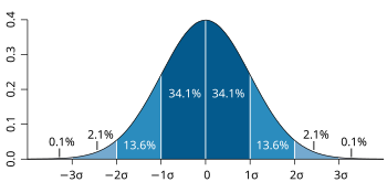
About 68% of values drawn from a normal distribution are within one standard deviation σ from the mean; about 95% of the values lie within two standard deviations; and about 99.7% are within three standard deviations.^[6] This fact is known as the 68–95–99.7 (empirical) rule, or the 3-sigma rule.

More precisely, the probability that a normal deviate lies in the range between ${\textstyle \mu -n\sigma }$ and ${\textstyle \mu +n\sigma }$ is given by $${\displaystyle F(\mu +n\sigma )-F(\mu -n\sigma )=\Phi (n)-\Phi (-n)=\operatorname {erf} \left({\frac {n}{\sqrt {2}}}\right).}$$ To 12 significant digits, the values for ${\textstyle n=1,2,\ldots ,6}$ are:

${\textstyle n}$	${\textstyle p=F(\mu +n\sigma )-F(\mu -n\sigma )}$	${\textstyle 1-p}$	${\textstyle {\text{or }}1{\text{ in }}(1-p)}$	OEIS
1	0.682689492137	0.317310507863	3 .15148718753	OEIS: A178647
2	0.954499736104	0.045500263896	21 .9778945080	OEIS: A110894
3	0.997300203937	0.002699796063	370 .398347345	OEIS: A270712
4	0.999936657516	0.000063342484	15787 .1927673
5	0.999999426697	0.000000573303	1744277 .89362
6	0.999999998027	0.000000001973	506797345 .897

For large ${\textstyle n}$, one can use the approximation ${\textstyle 1-p\approx {\frac {e^{-n^{2}/2}}{n{\sqrt {\pi /2}}}}}$.

The quantile function of a distribution is the inverse of the cumulative distribution function. The quantile function of the standard normal distribution is called the probit function, and can be expressed in terms of the inverse error function: $${\displaystyle \Phi ^{-1}(p)={\sqrt {2}}\operatorname {erf} ^{-1}(2p-1),\quad p\in (0,1).}$$ For a normal random variable with mean ${\textstyle \mu }$ and variance ${\textstyle \sigma ^{2}}$, the quantile function is $${\displaystyle F^{-1}(p)=\mu +\sigma \Phi ^{-1}(p)=\mu +\sigma {\sqrt {2}}\operatorname {erf} ^{-1}(2p-1),\quad p\in (0,1).}$$ The quantile ${\textstyle \Phi ^{-1}(p)}$ of the standard normal distribution is commonly denoted as ${\textstyle z_{p}}$. These values are used in hypothesis testing, construction of confidence intervals and Q–Q plots. A normal random variable ${\textstyle X}$ will exceed ${\textstyle \mu +z_{p}\sigma }$ with probability ${\textstyle 1-p}$, and will lie outside the interval ${\textstyle \mu \pm z_{p}\sigma }$ with probability ${\textstyle 2(1-p)}$. In particular, the quantile ${\textstyle z_{0.975}}$ is 1.96; therefore a normal random variable will lie outside the interval ${\textstyle \mu \pm 1.96\sigma }$ in only 5% of cases.

The following table gives the quantile ${\textstyle z_{p}}$ such that ${\textstyle X}$ will lie in the range ${\textstyle \mu \pm z_{p}\sigma }$ with a specified probability ${\textstyle p}$. These values are useful to determine tolerance interval for sample averages and other statistical estimators with normal (or asymptotically normal) distributions.^[15] The following table shows ${\textstyle {\sqrt {2}}\operatorname {erf} ^{-1}(p)=\Phi ^{-1}\left({\frac {p+1}{2}}\right)}$, not ${\textstyle \Phi ^{-1}(p)}$ as defined above.

${\textstyle p}$	${\textstyle z_{p}}$		${\textstyle p}$	${\textstyle z_{p}}$
0.80	1.281551565545		0.999	3.290526731492
0.90	1.644853626951		0.9999	3.890591886413
0.95	1.959963984540		0.99999	4.417173413469
0.98	2.326347874041		0.999999	4.891638475699
0.99	2.575829303549		0.9999999	5.326723886384
0.995	2.807033768344		0.99999999	5.730728868236
0.998	3.090232306168		0.999999999	6.109410204869

For small ${\textstyle p}$, the quantile function has the useful asymptotic expansion ${\textstyle \Phi ^{-1}(p)=-{\sqrt {\ln {\frac {1}{p^{2}}}-\ln \ln {\frac {1}{p^{2}}}-\ln(2\pi )}}+{\mathcal {o}}(1).}$^{[citation needed]}

The normal distribution is the only distribution whose cumulants beyond the first two (i.e., other than the mean and variance) are zero. It is also the continuous distribution with the maximum entropy for a specified mean and variance.^[16][17] Geary has shown, assuming that the mean and variance are finite, that the normal distribution is the only distribution where the mean and variance calculated from a set of independent draws are independent of each other.^[18][19]

The normal distribution is a subclass of the elliptical distributions. The normal distribution is symmetric about its mean, and is non-zero over the entire real line. As such it may not be a suitable model for variables that are inherently positive or strongly skewed, such as the weight of a person or the price of a share. Such variables may be better described by other distributions, such as the log-normal distribution or the Pareto distribution.

The value of the normal density is practically zero when the value ${\textstyle x}$ lies more than a few standard deviations away from the mean (e.g., a spread of three standard deviations covers all but 0.27% of the total distribution). Therefore, it may not be an appropriate model when one expects a significant fraction of outliers—values that lie many standard deviations away from the mean—and least squares and other statistical inference methods that are optimal for normally distributed variables often become highly unreliable when applied to such data. In those cases, a more heavy-tailed distribution should be assumed and the appropriate robust statistical inference methods applied.

The Gaussian distribution belongs to the family of stable distributions which are the attractors of sums of independent, identically distributed distributions whether or not the mean or variance is finite. Except for the Gaussian which is a limiting case, all stable distributions have heavy tails and infinite variance. It is one of the few distributions that are stable and that have probability density functions that can be expressed analytically, the others being the Cauchy distribution and the Lévy distribution.

The normal distribution with density ${\textstyle f(x)}$ (mean ${\textstyle \mu }$ and variance ${\textstyle \sigma ^{2}>0}$) has the following properties:

• It is symmetric around the point ${\textstyle x=\mu ,}$ which is at the same time the mode, the median and the mean of the distribution.^[20]
• It is unimodal: its first derivative is positive for ${\textstyle x<\mu ,}$ negative for ${\textstyle x>\mu ,}$ and zero only at ${\textstyle x=\mu .}$
• The area bounded by the curve and the ${\textstyle x}$-axis is unity (i.e. equal to one).
• Its first derivative is ${\textstyle f'(x)=-{\frac {x-\mu }{\sigma ^{2}}}f(x).}$
• Its second derivative is ${\textstyle f''(x)={\frac {(x-\mu )^{2}-\sigma ^{2}}{\sigma ^{4}}}f(x).}$
• Its density has two inflection points (where the second derivative of ${\textstyle f}$ is zero and changes sign), located one standard deviation away from the mean, namely at ${\textstyle x=\mu -\sigma }$ and ${\textstyle x=\mu +\sigma .}$^[20]
• Its density is log-concave.^[20]
• Its density is infinitely differentiable, indeed supersmooth of order 2.^[21]

Furthermore, the density ${\textstyle \varphi }$ of the standard normal distribution (i.e. ${\textstyle \mu =0}$ and ${\textstyle \sigma =1}$) also has the following properties:

• Its first derivative is ${\textstyle \varphi '(x)=-x\varphi (x).}$
• Its second derivative is ${\textstyle \varphi ''(x)=(x^{2}-1)\varphi (x)}$
• More generally, its nth derivative is ${\textstyle \varphi ^{(n)}(x)=(-1)^{n}\operatorname {He} _{n}(x)\varphi (x),}$ where ${\textstyle \operatorname {He} _{n}(x)}$ is the nth (probabilist) Hermite polynomial.^[22]
• The probability that a normally distributed variable ${\textstyle X}$ with known ${\textstyle \mu }$ and ${\textstyle \sigma ^{2}}$ is in a particular set, can be calculated by using the fact that the fraction ${\textstyle Z=(X-\mu )/\sigma }$ has a standard normal distribution.

The plain and absolute moments of a variable ${\textstyle X}$ are the expected values of ${\textstyle X^{p}}$ and ${\textstyle |X|^{p}}$, respectively. If the expected value ${\textstyle \mu }$ of ${\textstyle X}$ is zero, these parameters are called central moments; otherwise, these parameters are called non-central moments. Usually we are interested only in moments with integer order ${\textstyle \ p}$.

If ${\textstyle X}$ has a normal distribution, the non-central moments exist and are finite for any ${\textstyle p}$ whose real part is greater than −1. For any non-negative integer ${\textstyle p}$, the plain central moments are:^[23] $${\displaystyle \operatorname {E} \left[(X-\mu )^{p}\right]={\begin{cases}0&{\text{if }}p{\text{ is odd,}}\\\sigma ^{p}(p-1)!!&{\text{if }}p{\text{ is even.}}\end{cases}}}$$ Here ${\textstyle n!!}$ denotes the double factorial, that is, the product of all numbers from ${\textstyle n}$ to 1 that have the same parity as ${\textstyle n.}$

The central absolute moments coincide with plain moments for all even orders, but are nonzero for odd orders. For any non-negative integer ${\textstyle p,}$

$${\displaystyle {\begin{aligned}\operatorname {E} \left[|X-\mu |^{p}\right]&=\sigma ^{p}(p-1)!!\cdot {\begin{cases}{\sqrt {\frac {2}{\pi }}}&{\text{if }}p{\text{ is odd}}\\1&{\text{if }}p{\text{ is even}}\end{cases}}\\&=\sigma ^{p}\cdot {\frac {2^{p/2}\Gamma \left({\frac {p+1}{2}}\right)}{\sqrt {\pi }}}.\end{aligned}}}$$ The last formula is valid also for any non-integer ${\textstyle p>-1.}$ When the mean ${\textstyle \mu \neq 0,}$ the plain and absolute moments can be expressed in terms of confluent hypergeometric functions ${\textstyle {}_{1}F_{1}}$ and ${\textstyle U.}$^[24]

$${\displaystyle {\begin{aligned}\operatorname {E} \left[X^{p}\right]&=\sigma ^{p}\cdot (-i{\sqrt {2}})^{p}U\left(-{\frac {p}{2}},{\frac {1}{2}},-{\frac {1}{2}}\left({\frac {\mu }{\sigma }}\right)^{2}\right),\\\operatorname {E} \left[|X|^{p}\right]&=\sigma ^{p}\cdot 2^{p/2}{\frac {\Gamma \left({\frac {1+p}{2}}\right)}{\sqrt {\pi }}}{}_{1}F_{1}\left(-{\frac {p}{2}},{\frac {1}{2}},-{\frac {1}{2}}\left({\frac {\mu }{\sigma }}\right)^{2}\right).\end{aligned}}}$$

These expressions remain valid even if ${\textstyle p}$ is not an integer. See also generalized Hermite polynomials.

Order	Non-central moment	Central moment
1	${\textstyle \mu }$	${\textstyle 0}$
2	${\textstyle \mu ^{2}+\sigma ^{2}}$	${\textstyle \sigma ^{2}}$
3	${\textstyle \mu ^{3}+3\mu \sigma ^{2}}$	${\textstyle 0}$
4	${\textstyle \mu ^{4}+6\mu ^{2}\sigma ^{2}+3\sigma ^{4}}$	${\textstyle 3\sigma ^{4}}$
5	${\textstyle \mu ^{5}+10\mu ^{3}\sigma ^{2}+15\mu \sigma ^{4}}$	${\textstyle 0}$
6	${\textstyle \mu ^{6}+15\mu ^{4}\sigma ^{2}+45\mu ^{2}\sigma ^{4}+15\sigma ^{6}}$	${\textstyle 15\sigma ^{6}}$
7	${\textstyle \mu ^{7}+21\mu ^{5}\sigma ^{2}+105\mu ^{3}\sigma ^{4}+105\mu \sigma ^{6}}$	${\textstyle 0}$
8	${\textstyle \mu ^{8}+28\mu ^{6}\sigma ^{2}+210\mu ^{4}\sigma ^{4}+420\mu ^{2}\sigma ^{6}+105\sigma ^{8}}$	${\textstyle 105\sigma ^{8}}$

The expectation of ${\textstyle X}$ conditioned on the event that ${\textstyle X}$ lies in an interval ${\textstyle [a,b]}$ is given by $${\displaystyle \operatorname {E} \left[X\mid a<X<b\right]=\mu -\sigma ^{2}{\frac {f(b)-f(a)}{F(b)-F(a)}}\,,}$$ where ${\textstyle f}$ and ${\textstyle F}$ respectively are the density and the cumulative distribution function of ${\textstyle X}$. For ${\textstyle b=\infty }$ this is known as the inverse Mills ratio. Note that above, density ${\textstyle f}$ of ${\textstyle X}$ is used instead of standard normal density as in inverse Mills ratio, so here we have ${\textstyle \sigma ^{2}}$ instead of ${\textstyle \sigma }$.

The Fourier transform of a normal density ${\textstyle f}$ with mean ${\textstyle \mu }$ and variance ${\textstyle \sigma ^{2}}$ is^[25]

$${\displaystyle {\hat {f}}(t)=\int _{-\infty }^{\infty }f(x)e^{-itx}\,dx=e^{-i\mu t}e^{-{\frac {1}{2}}(\sigma t)^{2}}\,,}$$

where ${\textstyle i}$ is the imaginary unit. If the mean ${\textstyle \mu =0}$, the first factor is 1, and the Fourier transform is, apart from a constant factor, a normal density on the frequency domain, with mean 0 and variance ${\textstyle 1/\sigma ^{2}}$. In particular, the standard normal distribution ${\textstyle \varphi }$ is an eigenfunction of the Fourier transform.

In probability theory, the Fourier transform of the probability distribution of a real-valued random variable ${\textstyle X}$ is closely connected to the characteristic function ${\textstyle \varphi _{X}(t)}$ of that variable, which is defined as the expected value of ${\textstyle e^{itX}}$, as a function of the real variable ${\textstyle t}$ (the frequency parameter of the Fourier transform). This definition can be analytically extended to a complex-value variable ${\textstyle t}$.^[26] The relation between both is: $${\displaystyle \varphi _{X}(t)={\hat {f}}(-t)\,.}$$

The moment generating function of a real random variable ${\textstyle X}$ is the expected value of ${\textstyle e^{tX}}$, as a function of the real parameter ${\textstyle t}$. For a normal distribution with density ${\textstyle f}$, mean ${\textstyle \mu }$ and variance ${\textstyle \sigma ^{2}}$, the moment generating function exists and is equal to

$${\displaystyle M(t)=\operatorname {E} \left[e^{tX}\right]={\hat {f}}(it)=e^{\mu t}e^{\sigma ^{2}t^{2}/2}\,.}$$ For any ⁠${\displaystyle k}$⁠, the coefficient of ⁠${\displaystyle t^{k}/k!}$⁠ in the moment generating function (expressed as an exponential power series in ⁠${\displaystyle t}$⁠) is the normal distribution's expected value ⁠${\displaystyle E[X^{k}]}$⁠.

The cumulant generating function is the logarithm of the moment generating function, namely

$${\displaystyle g(t)=\ln M(t)=\mu t+{\tfrac {1}{2}}\sigma ^{2}t^{2}\,.}$$

The coefficients of this exponential power series define the cumulants, but because this is a quadratic polynomial in ⁠${\displaystyle t}$⁠, only the first two cumulants are nonzero, namely the mean ${\textstyle \mu }$ and the variance ⁠${\displaystyle \sigma ^{2}}$⁠.

Some authors prefer to instead work with the characteristic function E[e^itX] = e^{iμt − σ2t2/2} and ln E[e^itX] = iμt − ⁠1/2⁠σ²t².

Within Stein's method the Stein operator and class of a random variable ${\textstyle X\sim {\mathcal {N}}(\mu ,\sigma ^{2})}$ are ${\textstyle {\mathcal {A}}f(x)=\sigma ^{2}f'(x)-(x-\mu )f(x)}$ and ${\textstyle {\mathcal {F}}}$ the class of all absolutely continuous functions ${\textstyle f:\mathbb {R} \to \mathbb {R} {\mbox{ such that }}\mathbb {E} [|f'(X)|]<\infty }$.

In the limit when ${\textstyle \sigma ^{2}}$ tends to zero, the probability density ${\textstyle f(x)}$ eventually tends to zero at any ${\textstyle x\neq \mu }$, but grows without limit if ${\textstyle x=\mu }$, while its integral remains equal to 1. Therefore, the normal distribution cannot be defined as an ordinary function when ${\textstyle \sigma ^{2}=0}$.

However, one can define the normal distribution with zero variance as a generalized function; specifically, as a Dirac delta function ${\textstyle \delta }$ translated by the mean ${\textstyle \mu }$, that is ${\textstyle f(x)=\delta (x-\mu ).}$ Its cumulative distribution function is then the Heaviside step function translated by the mean ${\textstyle \mu }$, namely $${\displaystyle F(x)={\begin{cases}0&{\text{if }}x<\mu \\1&{\text{if }}x\geq \mu \,.\end{cases}}}$$

Of all probability distributions over the reals with a specified finite mean ${\textstyle \mu }$ and finite variance ${\textstyle \sigma ^{2}}$, the normal distribution ${\textstyle N(\mu ,\sigma ^{2})}$ is the one with maximum entropy.^[27] To see this, let ${\textstyle X}$ be a continuous random variable with probability density ${\textstyle f(x)}$. The entropy of ${\textstyle X}$ is defined as^[28][29][30] $${\displaystyle H(X)=-\int _{-\infty }^{\infty }f(x)\ln f(x)\,dx\,,}$$

where ${\textstyle f(x)\log f(x)}$ is understood to be zero whenever ${\textstyle f(x)=0}$. This functional can be maximized, subject to the constraints that the distribution is properly normalized and has a specified mean and variance, by using variational calculus. A function with three Lagrange multipliers is defined:

$${\displaystyle L=-\int _{-\infty }^{\infty }f(x)\ln f(x)\,dx-\lambda _{0}\left(1-\int _{-\infty }^{\infty }f(x)\,dx\right)-\lambda _{1}\left(\mu -\int _{-\infty }^{\infty }f(x)x\,dx\right)-\lambda _{2}\left(\sigma ^{2}-\int _{-\infty }^{\infty }f(x)(x-\mu )^{2}\,dx\right)\,.}$$

At maximum entropy, a small variation ${\textstyle \delta f(x)}$ about ${\textstyle f(x)}$ will produce a variation ${\textstyle \delta L}$ about ${\textstyle L}$ which is equal to 0:

$${\displaystyle 0=\delta L=\int _{-\infty }^{\infty }\delta f(x)\left(-\ln f(x)-1+\lambda _{0}+\lambda _{1}x+\lambda _{2}(x-\mu )^{2}\right)\,dx\,.}$$

Since this must hold for any small ${\textstyle \delta f(x)}$, the factor multiplying ${\textstyle \delta f(x)}$ must be zero, and solving for ${\textstyle f(x)}$ yields:

$${\displaystyle f(x)=\exp \left(-1+\lambda _{0}+\lambda _{1}x+\lambda _{2}(x-\mu )^{2}\right)\,.}$$

The Lagrange constraints that ${\textstyle f(x)}$ is properly normalized and has the specified mean and variance are satisfied if and only if ${\textstyle \lambda _{0}}$, ${\textstyle \lambda _{1}}$, and ${\textstyle \lambda _{2}}$ are chosen so that $${\displaystyle f(x)={\frac {1}{\sqrt {2\pi \sigma ^{2}}}}e^{-{\frac {(x-\mu )^{2}}{2\sigma ^{2}}}}\,.}$$ The entropy of a normal distribution ${\textstyle X\sim N(\mu ,\sigma ^{2})}$ is equal to $${\displaystyle H(X)={\tfrac {1}{2}}(1+\ln 2\sigma ^{2}\pi )\,,}$$ which is independent of the mean ${\textstyle \mu }$.

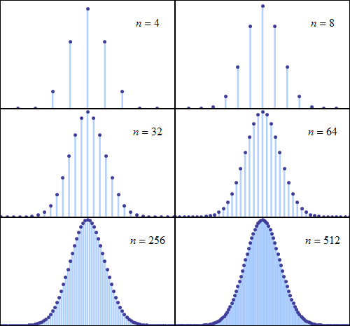
The central limit theorem states that under certain (fairly common) conditions, the sum of many random variables will have an approximately normal distribution. More specifically, where ${\textstyle X_{1},\ldots ,X_{n}}$ are independent and identically distributed random variables with the same arbitrary distribution, zero mean, and variance ${\textstyle \sigma ^{2}}$ and ${\textstyle Z}$ is their mean scaled by ${\textstyle {\sqrt {n}}}$ $${\displaystyle Z={\sqrt {n}}\left({\frac {1}{n}}\sum _{i=1}^{n}X_{i}\right)}$$ Then, as ${\textstyle n}$ increases, the probability distribution of ${\textstyle Z}$ will tend to the normal distribution with zero mean and variance ${\textstyle \sigma ^{2}}$.

The theorem can be extended to variables ${\textstyle (X_{i})}$ that are not independent and/or not identically distributed if certain constraints are placed on the degree of dependence and the moments of the distributions.

Many test statistics, scores, and estimators encountered in practice contain sums of certain random variables in them, and even more estimators can be represented as sums of random variables through the use of influence functions. The central limit theorem implies that those statistical parameters will have asymptotically normal distributions.

The central limit theorem also implies that certain distributions can be approximated by the normal distribution, for example:

• The binomial distribution ${\textstyle B(n,p)}$ is approximately normal with mean ${\textstyle np}$ and variance ${\textstyle np(1-p)}$ for large ${\textstyle n}$ and for ${\textstyle p}$ not too close to 0 or 1.
• The Poisson distribution with parameter ${\textstyle \lambda }$ is approximately normal with mean ${\textstyle \lambda }$ and variance ${\textstyle \lambda }$, for large values of ${\textstyle \lambda }$.^[38]
• The chi-squared distribution ${\textstyle \chi ^{2}(k)}$ is approximately normal with mean ${\textstyle k}$ and variance